Use Data from a Data Collection Project

Load the standard or distribution data from a local or remote data collection project.

Usage

dcf_data(
  variables = NULL,
  project = ".",
  data_format = NULL,
  project_type = "bundle",
  ...,
  unify = TRUE,
  only_selected = FALSE,
  cache = tempdir(),
  refresh = FALSE,
  verbose = TRUE
)

Arguments

variables: A character vector of variable names to be loaded, or a selected subset of a project data dictionary, as returned from dcf_variables.
project: Path to a local project, or the GitHub account and repository name ("{account_name}/{repo_name}") of a remote project.
data_format: The data format to select, between tall and wide. Useful if there are duplicate measure names between files of different formats.
project_type: Project type to select, between bundle and source.
...: Additional arguments passed to dcf_report.
unify: Logical; if FALSE, will return data as a list with entries for each file. Otherwise (by default), will attempt to combine the loaded data.
only_selected: Logical; if TRUE, will drop columns that were not included in variables, other than ID columns.
cache: Path to a directory in which to store downloaded files. Within this directory, the repository structure will be recreated within an account-named directory.
refresh: Logical; if TURE, will download files even if they exist in the cache.
verbose: Logical; if FALSE, will not show status messages.

Value

A list with entries for metadata (the datapackage resource entry for each file loaded) and data (a tibble or list of tibbles of the unified or separately loaded files).

Examples

# retrieve the full bundle file that includes the `epic_rsv` measure
bundle <- dcf_data(
  "epic_rsv",
  "dissc-yale/pophive_demo",
  data_format = "tall",
  verbose = FALSE
)
bundle$data
#> # A tibble: 55,889 × 6
#> # Groups:   measure [5]
#>    geography time       measure              value value_scaled source_file     
#>    <chr>     <date>     <chr>                <dbl>        <dbl> <chr>           
#>  1 0         2023-01-01 epic_all_encounters 854874        75.4  data/bundle_tal…
#>  2 0         2023-01-01 epic_rsv              2582        20.5  data/bundle_tal…
#>  3 0         2023-01-08 epic_all_encounters 804025        70.9  data/bundle_tal…
#>  4 0         2023-01-08 epic_rsv              1659        13.2  data/bundle_tal…
#>  5 0         2023-01-15 epic_all_encounters 808560        71.3  data/bundle_tal…
#>  6 0         2023-01-15 epic_rsv              1254         9.94 data/bundle_tal…
#>  7 0         2023-01-22 epic_all_encounters 806785        71.1  data/bundle_tal…
#>  8 0         2023-01-22 epic_rsv              1069         8.47 data/bundle_tal…
#>  9 0         2023-01-29 epic_all_encounters 801378        70.7  data/bundle_tal…
#> 10 0         2023-01-29 epic_rsv               852         6.74 data/bundle_tal…
#> # ℹ 55,879 more rows

if (require("ggplot2", quietly = TRUE)) {
  # extract short names from metadata
  labels <- vapply(
    bundle$metadata[[1L]]$schema$fields[[3L]]$info$levels,
    function(measure) measure$info$short_name,
    ""
  )

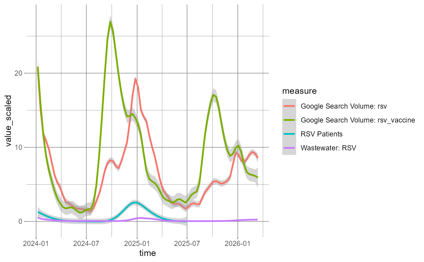
  # show trends from different measures over time
  bundle$data |>
    dplyr::filter(
      time >= as.Date("2024-01-01"),
      measure != "epic_all_encounters"
    ) |>
    dplyr::mutate(measure = labels[measure]) |>
    ggplot(aes(x = time, y = value_scaled, color = measure)) +
    theme_dark() %+replace%
    theme(panel.background = element_rect(fill = FALSE, color = FALSE)) +
    geom_smooth(
      method = "gam",
      formula = y ~ s(x, bs = "cs", k = 50L)
    )
}

Use Data from a Data Collection Project

Usage

Arguments

Value

See also

Examples